Not all the water that reaches a landscape stays in the soil or ends up in a river. Part of it returns to the atmosphere, through evaporation from the surface and transpiration from vegetation. Reading that exchange helps explain how a landscape works and how it changes from season to season.
Atlas’s Evapotranspiration (ET) indicator estimates that transfer of water, pixel by pixel, in millimeters per day (mm/day). It combines satellite and weather data in a surface energy balance, calibrated with the METRIC method (Allen et al., 2007). In Atlas you read it as annual and seasonal averages, a monthly chart and a map with values by location.
What it calculates: actual evapotranspiration
The indicator delivers actual evapotranspiration (ETa): the water that, according to the model, actually leaves the soil and vegetation for the atmosphere, limited by the water available.
Reference evapotranspiration (ETr) represents something else: the atmosphere’s demand on a well-watered reference crop. The model uses it as a yardstick. It estimates what fraction of that demand each pixel meets and uses it to obtain the daily result.
A value in mm/day describes the estimated transfer from the surface to the atmosphere. Water drawn from a well and irrigation applied are measured by other means. One millimeter equals one liter per square meter. The daily unit expresses a rate, useful for comparing periods, and is distinct from an annual total.
Lemu’s verdict: compare patterns, with clear limits
ET is useful for comparing zones, seasons and years within a region, and for identifying where the landscape returns more or less water to the atmosphere. It adds context to the analysis of irrigated and rainfed land, to a restoration project or to a review of water availability.
Its strength is combining spatial detail with a calibration for each scene, and it is designed for reading trends and contrasts. When an absolute value must be auditable, ET is complemented by a flux measurement or an official water balance.
What the indicator shows in Atlas
In a zone where the indicator has been calculated, you will find Evapotranspiration in the Climate section. The screen lets you choose the year and the analysis surface.
| Element | What you can look up |
|---|---|
| Summary | The annual average and the summer, autumn, winter and spring averages, in mm/day. |
| Analysis dimensions (Analysis Dimension in the interface) | The Year, Summer, Autumn, Winter and Spring views that organize the query. |
| Monthly chart | Evapotranspiration month by month for the selected year. |
| Map and legend | The spatial distribution of the values and their scale in mm/day. |
| Detail of a geometry | The value of the element selected on the map, which differs from the average for the whole zone. |
A simple route: choose a year, review the seasonal averages and use the map to locate differences within the area analyzed. The time views place each value in context, because a summer value and a winter value reflect different conditions.
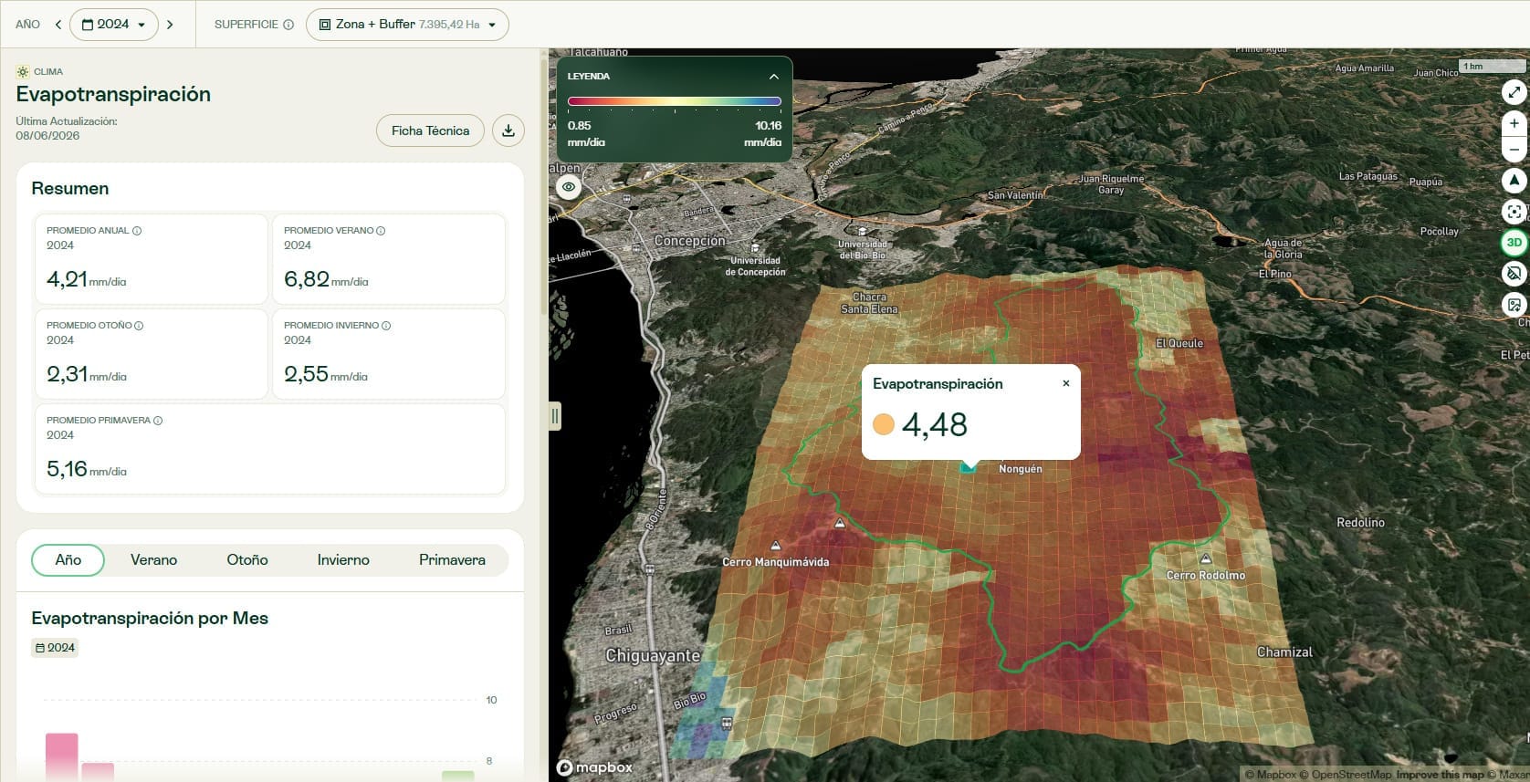
Averages are still expressed in mm/day. They are the mean daily rate for the year or the season, which differs from the total water evapotranspired over that period. Likewise, the number that appears when you select a geometry applies only to that element of the map.
How the estimate is built
Satellites do not measure evapotranspiration directly. They record surface temperature and reflectance. The model uses those observations to estimate how energy is split between heating the soil, heating the air and evaporating water.
The method combines a surface energy balance with anchor calibration based on the METRIC method. In each scene, cold and hot surface references are chosen, and each is assigned a fraction of reference evapotranspiration according to its vegetation. That way the model does not assume that the greenest reference in a desert behaves like a well-irrigated crop, or that the hottest reference in a forest stops transpiring.
The calculation follows six steps:
- Prepare the surface variables.
- Correct temperature for elevation.
- Estimate the available energy.
- Select and calibrate the anchors.
- Estimate the heat transferred to the air.
- Scale instantaneous evapotranspiration to a daily value.
Calibration and map generation use the same aerodynamic calculation. The model also applies a minimum roughness to bare-soil areas.
| Specification | Description |
|---|---|
| Variable | Estimated daily actual evapotranspiration, in mm/day, with a monthly average. |
| Spatial output | 30 m grid. |
| Observation frequency | Each valid Landsat 8/9 scene. With both satellites, the nominal revisit is about 8 days. |
| Satellite data | Landsat 8/9 Collection 2 Level 2, and Sentinel-2 for vegetation information. |
| Weather | Hourly ERA5-Land. |
| Topography | NASA SRTM v3. |
| Method output range | 0 to 15 mm/day. |
| Calculation area | The study zone plus a buffer that follows the shape of its sectors. The combined area is 1.3 times the area of the zone. |
The 30 meters describe the output grid; native resolution varies by source. The technical sheet details Landsat thermal data at 100 meters, resampled to 30, and ERA5-Land weather at about 9 kilometers.
The sources are global in scope, but SRTM v3 only covers 60° N to 56° S, and the documentation does not specify an alternative elevation source outside that range. So check availability for each zone with Lemu, without assuming unrestricted coverage.
A daily rate depends on the scenes available
The calculation produces a daily estimate for each valid scene. The monthly average uses only the days with valid Landsat observations, and cloud cover can reduce how many there are.
If a month has no valid scene, it has no data: for now, those gaps are not interpolated. An empty month does not mean zero evapotranspiration. Scaling to a daily rate cannot see through clouds.
What the comparison with OpenET shows
Lemu Earth Science documents a comparison with OpenET at 10 sites in the United States, covering desert, forest and irrigated agriculture, for April to August 2024. OpenET, the ensemble of reference models used in that comparison, also delivers model-based estimates.
In that evaluation, Lemu Earth Science reports a mean error of about 18%, with 29% at the site with the largest error. These results describe the comparison at those 10 sites. The error for a particular month, pixel, country or customer zone may differ.
Strengths and limitations when using ET
The indicator lets you review differences at the scale of a single property and compare areas with a per-scene calibration, using satellite and weather data.
Reading it requires taking climate, season and land cover into account. High ET indicates a greater estimated transfer of water to the atmosphere; low ET can reflect dry soil, less vegetation or a water deficit. A single value is not a complete diagnosis of the state of an ecosystem.
The documentation identifies specific limitations:
- It depends on clear-sky scenes.
- It can overestimate forest evapotranspiration in spring.
- It can underestimate irrigation in midsummer, when ERA5-Land winds are low.
- The weather data do not capture all local detail.
- It provides no per-pixel uncertainty.
The technical sheet also notes simplifications in the aerodynamic calculation and in the daily scaling.
Questions it can help answer
Zone and surroundings. Contrasting the evapotranspiration of a property with that of the surrounding landscape lets you explore differences in water use. The technical sheet proposes this reading as an input for analyzing dependencies and impacts on water.
Restoration and reforestation. Comparing the same season across years helps track changes linked to the recovery of vegetation cover, without assuming that a higher value is always better.
Irrigated and rainfed land. Reviewing patterns on irrigated properties and neighboring areas guides an assessment of relative water use and helps decide where to look more closely.
Possible water deficit. The model relates ETa to reference demand through the reference evapotranspiration fraction (ETrF), an internal variable of the method. Lower transpiration than expected can point to a review of water stress.
When to complement it with another source
MODIS MOD16 offers an alternative for long series and large regions, at a coarser 500-meter resolution. OpenET, the reference in this evaluation, can complement the analysis where it has coverage. Ground measurements, such as flux towers or lysimeters, remain necessary when an auditable absolute volume is required.
The goal is a spatial estimate that lets you compare, recognize patterns and guide the next review, with its limits in view. The other water questions are answered by combining sources.
Look up the indicator
Open Atlas and, in a zone where the indicator has been calculated, go to Climate → Evapotranspiration. Choose a year and surface, review the summary and check the map values. To find out whether the calculation is available for your zones, or for help interpreting it, contact your Lemu team.
See what else is new in Atlas 1.6.0.
Method and sources
The description of the method and the evaluation results come from Lemu Earth Science’s documentation for this indicator. Its methodological references are:
- Allen, R. G., Tasumi, M. and Trezza, R. (2007). Satellite-based energy balance for mapping evapotranspiration with internalized calibration (METRIC): Model. Method reference.
- Allen, R. G., Pereira, L. S., Raes, D. and Smith, M. (1998). Crop evapotranspiration: Guidelines for computing crop water requirements. FAO Irrigation and Drainage Paper 56.
- Liang, S. (2001). Narrowband to broadband conversions of land surface albedo I: Algorithms. Reference.
- Wei, J., Zhang, Z., Liu, B., Cui, Y., Luo, Y. and Tang, X. (2025). Breaking the zero-flux paradigm: An iterative surface energy balance framework for enhanced cold pixel characterization. Reference.
Data: USGS Landsat 8/9 Collection 2 Level 2; Copernicus Sentinel-2 L2A; NASA SRTM v3; ECMWF ERA5-Land.